
Napa - Adaptive Partitioning for Distributed Queries
Efficient query execution in distributed data warehouses depends on how well the workload is balanced across nodes. Napa improves performance by dynamically partitioning data at query time, adapting to each query’s needs instead of relying on fixed partitions. It uses a progressive approach designed to be “good enough” thereby balancing partitioning time and performance.
A typical data warehouse consists of a data scattered across many different nodes. Any given query might require reading from many nodes to provide a response. To achieve low latency, multiple query nodes work in parallel, partially aggregating data on each node before merging the results into a consolidated response for the user.
For this technique to be effective, the load must be evenly distributed across all query nodes. Otherwise, some nodes might process millions of rows, while others handle just a few. The total query time depends on the slowest node.
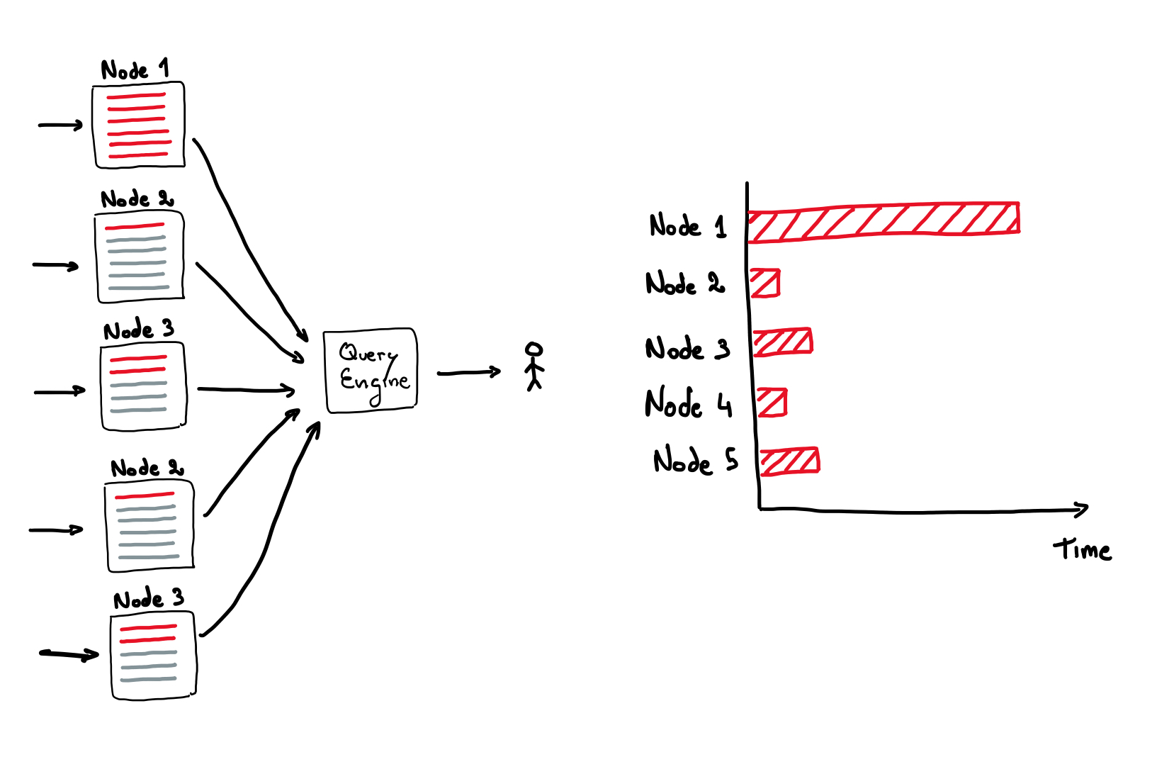
You might think that adding more query nodes would speed things up, but if the load distribution is skewed, you won’t see much performance improvement. The query will still be stuck waiting for the slowest node to finish reading its data while other nodes sit idle.
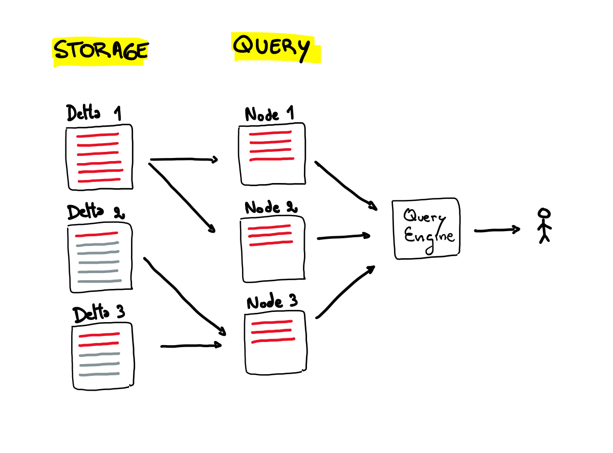
A common solution to this problem is sharding the data at write time based on an attribute. As data is ingested, it is partitioned based on this attribute’s value (e.g., timestamp, user ID, region). At query time, workers read only the partitions relevant to their assigned key range.
This approach works well if queries align with the chosen partitioning scheme, but inevitably, some queries won’t fit the predefined partitioning, making them slower and inefficient.
Instead of relying on fixed partitions at write time, Napa dynamically calculates data partitioning at query time. This allows the system to:
- Adapt the partitioning scheme to match the specific query predicates.
- Vary partition granularity based on how much data matches the query.
For example, let’s say the data is partitioned by time, and your query spans three days. If most of the results are from day one, while days two and three contain very little data, Napa’s algorithm automatically assigns fine-grained partitions for day one while using coarse-grained partitions for days two and three.
How it works
At a high level the query algorithm can be divided in the following stages:
- Search the B-Tree
- Calculate partitioning
- Retrieve data and compute the query result.
The naive solution would be to traverse the entire index space exhaustively, and then split the matches across all query nodes perfectly evenly. This would produce the optimal partitioning scheme. However, in the search for “perfection” the algorithm might end up exhausting the latency budget allotted for the full query.
We need to be able to calculate a “good enough” partitioning scheme in a bounded amount of time, so the rest of the time can be spent reading the data and computing the result.
To achieve this, Napa’s enriches the B-Trees indices with statistics on data size in a hierarchical manner. The query engine uses this information to estimate the input data size of the query and calculate the partitions.
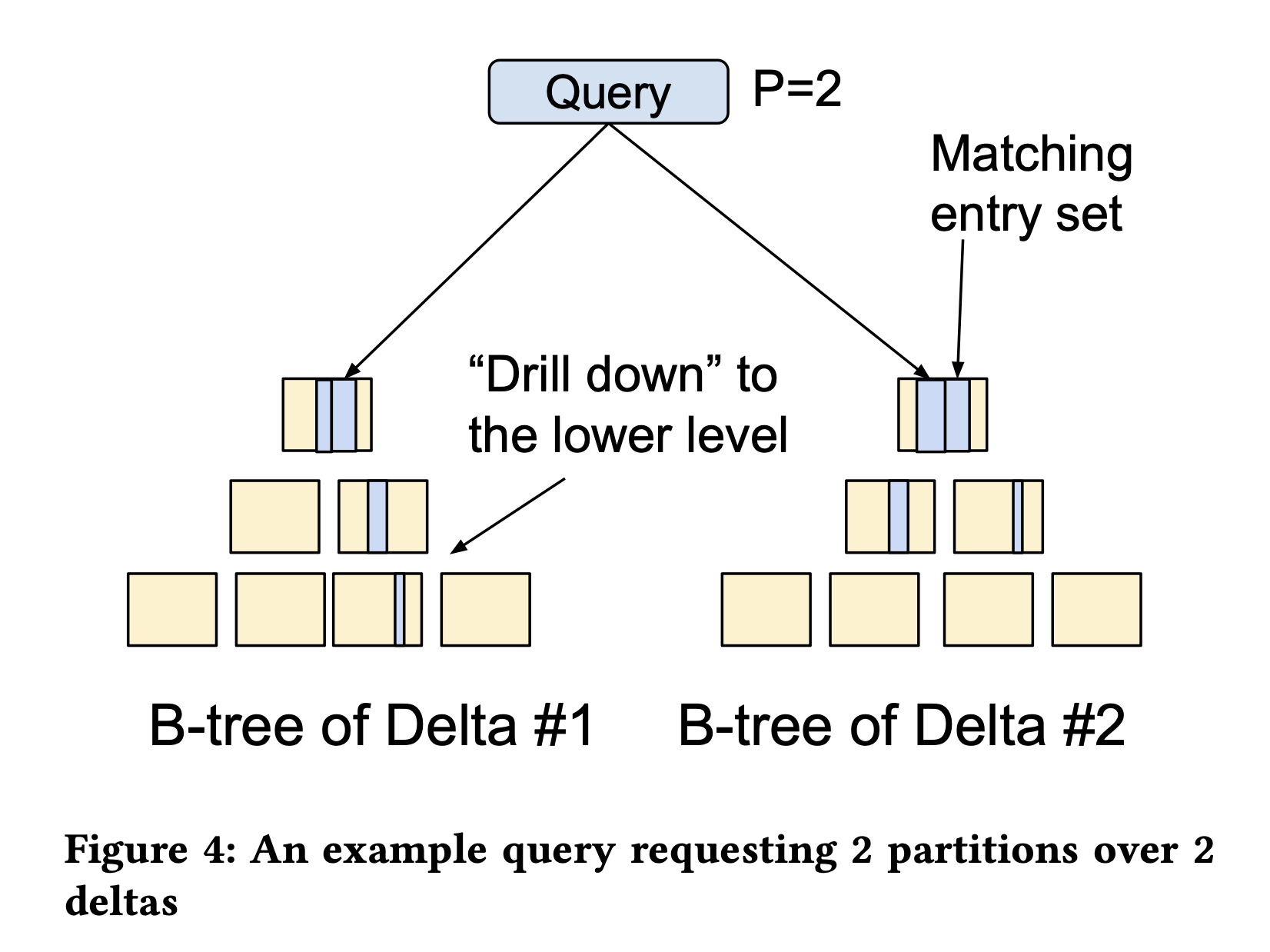
The algorithm uses an error margin ratio parameter 𝜃 to control how good is good enough. To calculate partitioning it traverses the index retrieving the size estimate starting from the root of the B-Tree.
A candidate split point is then selected. The split point will inevitably divide a delta in two making the size information imprecise because we don’t know what the data skew inside the delta is.
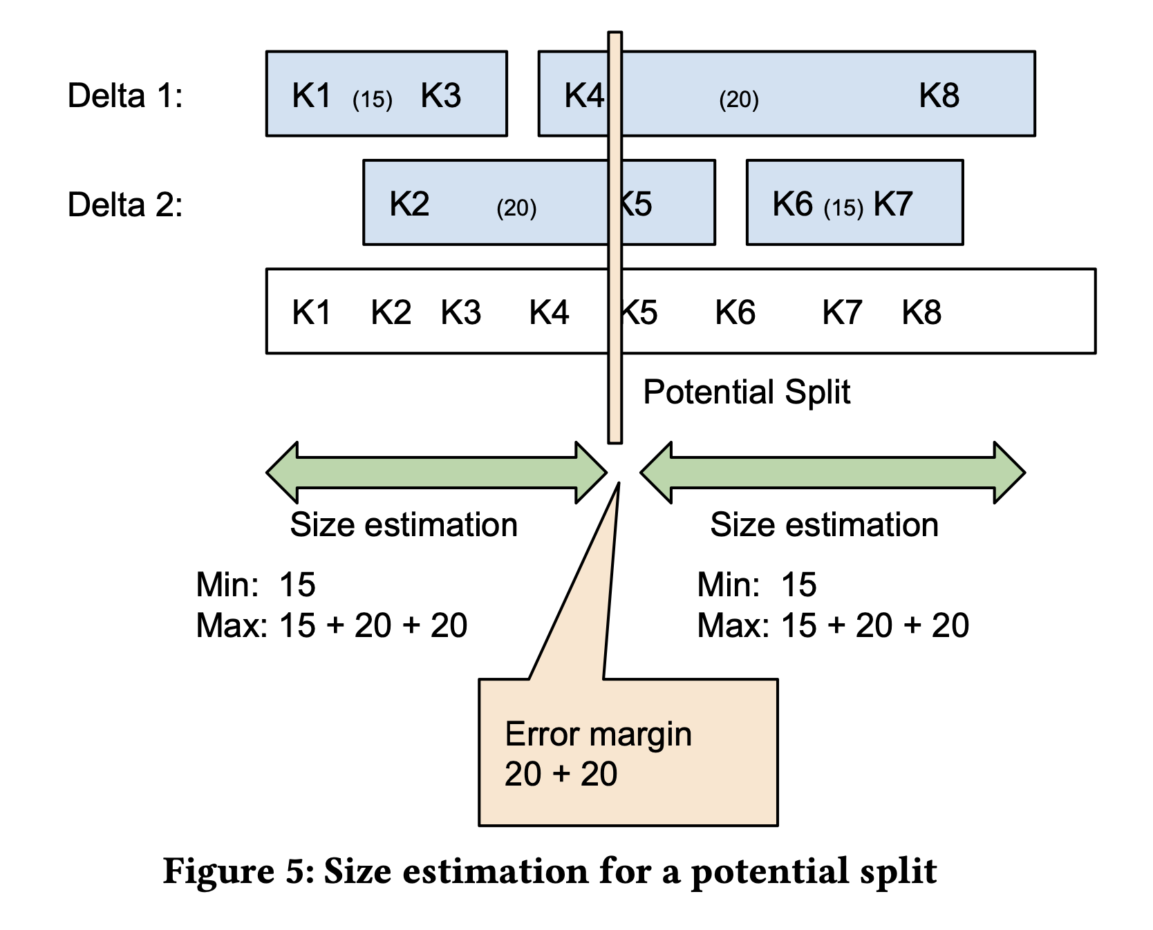
Using the candidate split point, the algorithm calculates the error margin and compares it with 𝜃. If the error margin is too high, the algorithm drills down into the next level of the B-Tree to refine the partitioning. This process continues selectively, only descending further in the tree where finer partitions are needed.
By using this approach, the algorithm can spend more time and produce finer grained partitions on deltas where there are more hits, and use the faster coarse estimation on more sparse deltas.
Tuning for Different Query Types
Interestingly, the same algorithm can be used for both online queries and large batch use cases. Different margin error 𝜃 can be used for different use cases:
- For sub-second query latency they use 𝜃 = 1 for a bounded error rate.
- For large batch use cases they use 𝜃 = 0 because they can spend extra time to calculate the most accurate partition.
